Given that Hadoop is a framework for processing data, is it better than standard relational databases, the workhorse of data processing in most of today’s applications? Here are some key difference between the two :
Main memory graph mining algorithms typically face two problems with respect to scalability.Graphs could be larger than the main memory available and hence cannot be loaded into main memory or the algorithm could be computationally expensive and the computation space required is more than the available main memory. Relational Databases are known for their ability to handle massive data sets and hence can be used to overcome this limitation.A second approach could be to use the MapReduce framework which can parallelize the graph query across huge datasets using a large number of computers (nodes). A recent benchmark study using a popular open source MR implementation and two parallel RDBMSs showed that the RDBMSs are substantially faster than the MR system once the data is loaded. This study used the Grep task from the original MR (MapReduce) paper to compare performance trade-offs between parallel RDBMSs and MR system. The graph problem I researched for my study was that of SubGraph Pattern Matching.
Subgraph Query
The subgraph search operation can be described as follows:
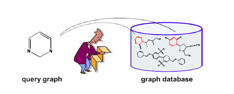
Given a graph database D = {g1, g2, .. , gn} and a graph query q, to answer the query is to find all graphs that contain q in D.
- SQL (structured query language) is by design targeted at structured data. Many of Hadoop’s initial applications deal with unstructured data such as text. From this perspective Hadoop provides a more general paradigm than SQL.
- In principle, SQL and Hadoop can be complementary, as SQL is a query language which can be implemented on top of Hadoop as the execution engine.
- But in practice, SQL databases tend to refer to a whole set of technologies, with several dominant vendors, optimized for a historical set of applications. Relational Databases are hence very mature, they are fault tolerant and provide rich parallelism.
- Hadoop is designed for offline processing and analysis of large-scale data. It doesn’t work for random reading and writing of a few records, which is the type of load for online transaction processing.
- SCALE-OUT INSTEAD OF SCALE-UP : Studies show that scale-up (use a more powerful Server) is more cost-effective for many real-world jobs which today use scale-out. However, clearly there is a job size beyond which scale out (use more Servers) becomes a better option. This “cross-over” point is job-specific.
Main memory graph mining algorithms typically face two problems with respect to scalability.Graphs could be larger than the main memory available and hence cannot be loaded into main memory or the algorithm could be computationally expensive and the computation space required is more than the available main memory. Relational Databases are known for their ability to handle massive data sets and hence can be used to overcome this limitation.A second approach could be to use the MapReduce framework which can parallelize the graph query across huge datasets using a large number of computers (nodes). A recent benchmark study using a popular open source MR implementation and two parallel RDBMSs showed that the RDBMSs are substantially faster than the MR system once the data is loaded. This study used the Grep task from the original MR (MapReduce) paper to compare performance trade-offs between parallel RDBMSs and MR system. The graph problem I researched for my study was that of SubGraph Pattern Matching.
Subgraph Query
The subgraph search operation can be described as follows:
Given a graph database D = {g1, g2, .. , gn} and a graph query q, to answer the query is to find all graphs that contain q in D.
Graph Encoding Schemes in Relational Databases
An efficient and suitable encoding for each graph member gi in the graph database D can make a big difference in the query execution performance. We first use the popular Vertex-Edge mapping scheme as a simple relational storage scheme for storing our targeting directed labeled graphs. In this mapping scheme, each graph database member gi is assigned a unique identity graphID. Each vertex is assigned a sequence number (vertexID) inside its graph. Each vertex is represented by one tuple in a single table (Vertices table) which stores all vertices of the graph database. Each vertex is identified by the graphID for which the vertex belongs to and the vertex ID. Additionally, each vertex has an additional attribute to store the vertex label. Similarly, all edges of the graph database are stored in a single table (Edges table) where each edge is represented by a single tuple in this table. So the Vertex-Edge mapping scheme can be described as:
Vertices(graphID, vertexID, vertexLabel)
Edges(graphID, sVertex, dVertex, edgeLabel)
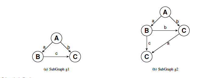
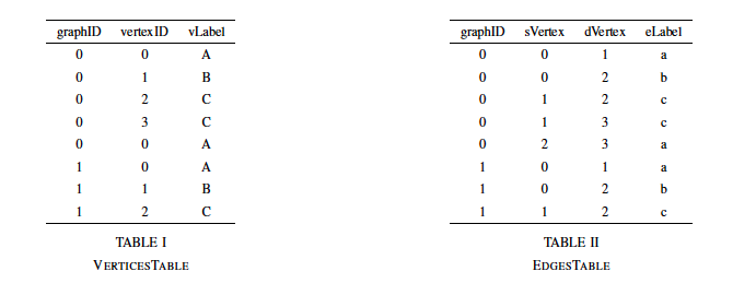
The figure above shows two sample graphs g1 and g2 in the graph database. The graphs are then stored in the database using Vertex-Edge mapping scheme as shown in Table: I and Table: II. A sub-graph query q consists of a set of vertices QV with size equal m and a set of edges QE equal n .
Let us now search for the following subgraph in the database:
Let us now search for the following subgraph in the database:
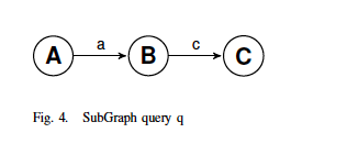
The rather simple SQL query to search the subgraph above (its a really simple graph) in the graph database could look like:
select distinct V1.graphID,V1.vLabel,V2.vLabel,V3.vLabel
from VerticesTable as V1, VerticesTable as V2, VerticesTable as V3,
EdgesTable as E1, EdgesTable as E2
where ((V1.graphID = V2.graphID) and (V1.graphID = V3.graphID))
and ((V1.graphID = E1.graphID) and (V1.graphID = E2.graphID))
and ((V1.vertexID = E1.sVertex) AND (V2.vertexID = E1.dVertex)
and (V2.vertexID = E2.sVertex) and (V3.vertexID = E2.dVertex))
and (V1.vLabel = ’A’ and V2.vLabel = ’B’ and V3.vLabel = ’C’)
and (E1.eLabel = ’a’ and E2.eLabel = ’c’)
ORDER BY V1.graphID
While the query above can be optimized, nothing changes the fact that the SQL query involves (m + n) joins of Vertices and Edges tables instances. Hence, although this query can be efficiently used with relatively small sub-graph search queries, medium size or large sub-graph queries will become too long and complex to write.
Hence, using the Vertex-Edge mapping scheme, the number of join operations between the encoding relations is equal to m + n . However, we may consider another encoding scheme, namely the Edge-Edge mapping scheme, which reduces to only n join operations. The relational storage scheme of the Edge-Edge mapping is described as follows:
EdgeEdge(graphID, edgeID,eLabel, sVertex, dVertex, sLabel, dLabel)
The Edge-Edge mapping scheme, though more efficient may suffer from update anomalies (as we store all the information in a single EdgeEdge table).
MAP REDUCE
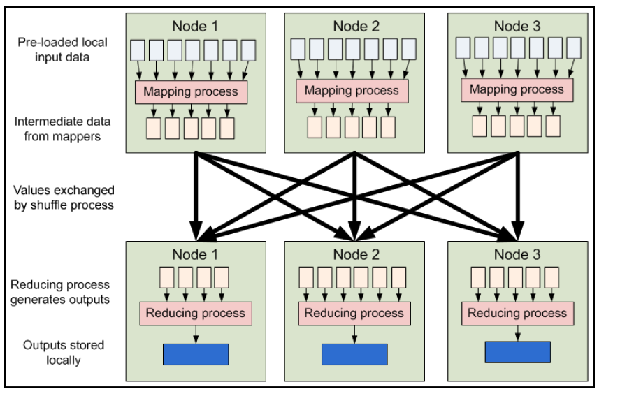
At Google, MapReduce is used for Index construction for Google Search, Article clustering for Google News, Statistical machine translation and many other applications.Hadoop Map/Reduce is a software framework for easily writing applications which process vast amounts of data (multi-terabyte data-sets) in-parallel on large clusters (thousands of nodes) of commodity hardware in a reliable, fault-tolerant manner.A Map/Reduce job usually splits the input data-set into independent chunks which are processed by the map tasks in a completely parallel manner. The framework sorts the outputs of the maps, which are then input to the reduce tasks. Typically both the input and the output of the job are stored in a file-system. The framework takes care of scheduling tasks, monitoring them and re-executes the failed tasks. Typically the compute nodes and the storage nodes are the same, that is, the Map/Reduce framework and the Hadoop Distributed File System (see HDFS Architecture ) are running on the same set of nodes. This configuration allows the framework to effectively schedule tasks on the nodes where data is already present, resulting in very high aggregate bandwidth across the cluster.
The Map/Reduce framework consists of a single master JobTracker and one slave TaskTracker per clusternode. The master is responsible for scheduling the jobs’ component tasks on the slaves, monitoring them and re-executing the failed tasks. The slaves execute the tasks as directed by the master.
select distinct V1.graphID,V1.vLabel,V2.vLabel,V3.vLabel
from VerticesTable as V1, VerticesTable as V2, VerticesTable as V3,
EdgesTable as E1, EdgesTable as E2
where ((V1.graphID = V2.graphID) and (V1.graphID = V3.graphID))
and ((V1.graphID = E1.graphID) and (V1.graphID = E2.graphID))
and ((V1.vertexID = E1.sVertex) AND (V2.vertexID = E1.dVertex)
and (V2.vertexID = E2.sVertex) and (V3.vertexID = E2.dVertex))
and (V1.vLabel = ’A’ and V2.vLabel = ’B’ and V3.vLabel = ’C’)
and (E1.eLabel = ’a’ and E2.eLabel = ’c’)
ORDER BY V1.graphID
While the query above can be optimized, nothing changes the fact that the SQL query involves (m + n) joins of Vertices and Edges tables instances. Hence, although this query can be efficiently used with relatively small sub-graph search queries, medium size or large sub-graph queries will become too long and complex to write.
Hence, using the Vertex-Edge mapping scheme, the number of join operations between the encoding relations is equal to m + n . However, we may consider another encoding scheme, namely the Edge-Edge mapping scheme, which reduces to only n join operations. The relational storage scheme of the Edge-Edge mapping is described as follows:
EdgeEdge(graphID, edgeID,eLabel, sVertex, dVertex, sLabel, dLabel)
The Edge-Edge mapping scheme, though more efficient may suffer from update anomalies (as we store all the information in a single EdgeEdge table).
MAP REDUCE
At Google, MapReduce is used for Index construction for Google Search, Article clustering for Google News, Statistical machine translation and many other applications.Hadoop Map/Reduce is a software framework for easily writing applications which process vast amounts of data (multi-terabyte data-sets) in-parallel on large clusters (thousands of nodes) of commodity hardware in a reliable, fault-tolerant manner.A Map/Reduce job usually splits the input data-set into independent chunks which are processed by the map tasks in a completely parallel manner. The framework sorts the outputs of the maps, which are then input to the reduce tasks. Typically both the input and the output of the job are stored in a file-system. The framework takes care of scheduling tasks, monitoring them and re-executes the failed tasks. Typically the compute nodes and the storage nodes are the same, that is, the Map/Reduce framework and the Hadoop Distributed File System (see HDFS Architecture ) are running on the same set of nodes. This configuration allows the framework to effectively schedule tasks on the nodes where data is already present, resulting in very high aggregate bandwidth across the cluster.
The Map/Reduce framework consists of a single master JobTracker and one slave TaskTracker per clusternode. The master is responsible for scheduling the jobs’ component tasks on the slaves, monitoring them and re-executing the failed tasks. The slaves execute the tasks as directed by the master.
Minimally, applications specify the input/output locations and supply map and reduce functions via implementations of appropriate interfaces and/or abstract-classes. These, and other job parameters, comprise the job configuration. The Hadoop job client then submits the job (jar/executable etc.) and configuration to the JobTracker which then assumes the responsibility of distributing the software/configuration to the slaves, scheduling tasks and monitoring them, providing status and diagnostic information to the job-client.
SUBGRAPH PATTERN MATCHING IN MAP REDUCE
In this section, I'll give an overview of our subgraph search approach implemented in the MapReduce framework. The main idea is to build inverted edge indexes for the graphs in the database and to use these indexes to process queries :
Offline Indexing
We use the graph database stored in the Edge-Edge schema format for building the index. The graph is exported
from the relational database system into a comma delimited text file. In the text file, each edge of a graph is
represented as a (graphID=sLabel; dLabel) pair where graphID represents the graph containing the indexed
edge, (sLabel; dLabel) consists of the labels of the edges two end vertices. The index is built in two stages
as shown in figure below:
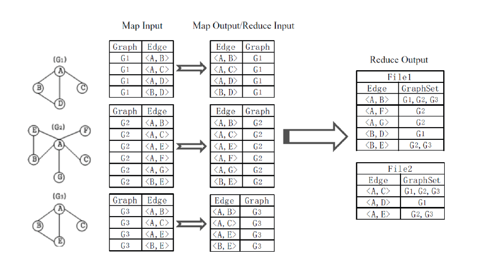
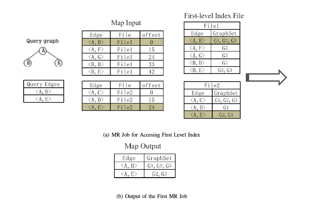
- In the first stage, each graphID=sLabel; dLabel is reversed by the Map function to output a sLabel; dLabel=GraphNo pair. In the Reduce function, pairs with identical EdgeLabel are aggregated together, and the Reduce function generates an sLabel; dLabel=GraphSet pair where the GraphSet contains the set of graphID’s for a particular edge.
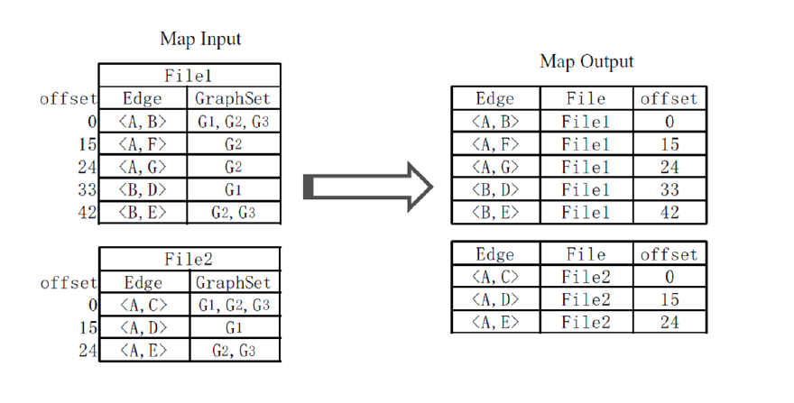
When the first MapReduce job finishes, a second MapReduce job is launched to build the second-level index.
The second-level index constructs the mappings between edges and their offsets in the first-level index files. Each of the firstlevel index files is treated as an input for a Mapper of the second MapReduce job. When a EdgeLabel/GraphSet pair in any of the first-level index files is processed by the Map function, the file name and the offset of the current inverted index entry in the first-level index files are recorded. Then the Map function outputs an sLabel; dLabel=FileName;Offset pair.
First and Second Level Index :
Online Querying
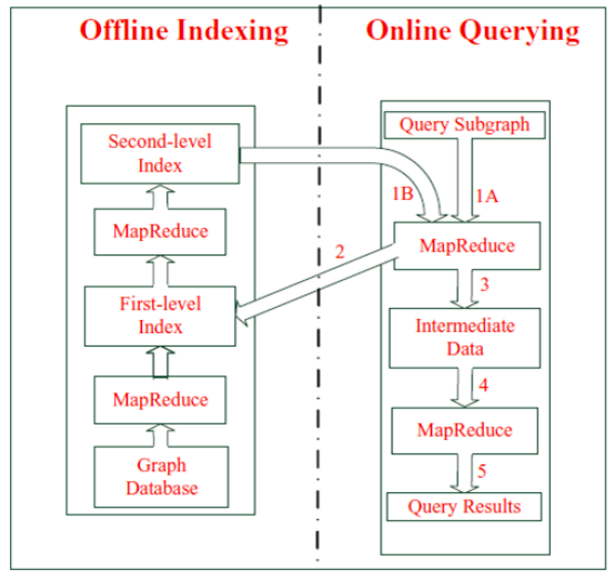
When a query is issued, two MapReduce jobs are initiated to process the subgraph query. The logics of executing
graph query are presented in figure below. The first MapReduce job is used to retrieve the inverted edge index entries
whose corresponding edges are contained in the query graph. The second MapReduce job performs a series of set
intersection operations to generate the final query results.
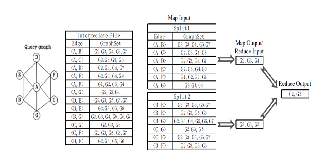
Evaluation on Hadoop
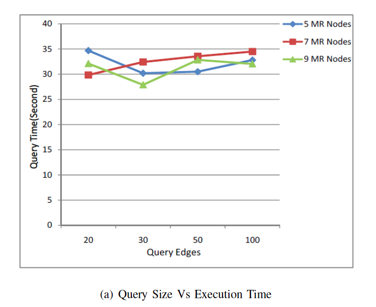
In hadoop we were interested to see how the size of the input Query Graph affects the Overall Query Time. We were also interested to see if adding more MapReduce nodes and tasks would help reduce the query time or not. It is interesting to note that in hadoop the number of map tasks for a given job is driven by the number of input splits and not by the mapred.map.tasks parameter. If the number of query edges increases, the query time should increase, since more time will be spent on checking whether the EdgeLabels of an entry in the second-level index is contained in the query graph. However, as we can see from figure below, the query time sometimes decreases as the number of query edges increases.
The reason behind this is that the computing cost spent on checking is minor, compared with that of data distribution and the subsequent graph set intersection operations. As for the MapReduce job that performs graph set intersection operations, the majority of the execution time is spent on the Reducer. The Reducer performs intersection operations on all the outputs of the preceding Mappers. When the input query is small, the input of the Reducer is of relatively of large size, and thus it takes the Reducer much time to finish the intersection operation on the graph sets. When the query graph contains more edges, more Mappers will be initiated to perform local graph set intersection operations, and each Mapper gets more graph sets as inputs.So the outputs of the Mappers and thus the input of the Reducer may become smaller and it take less time to finish the execution. Another interesting observation is that increasing the number of nodes has little affect on the overall query execution time. For our dataset, hadoop setup with 7 nodes performed the best.
 RSS Feed
